


")
Overview
SigmaPlot Helps You Quickly Create Exact Graphs
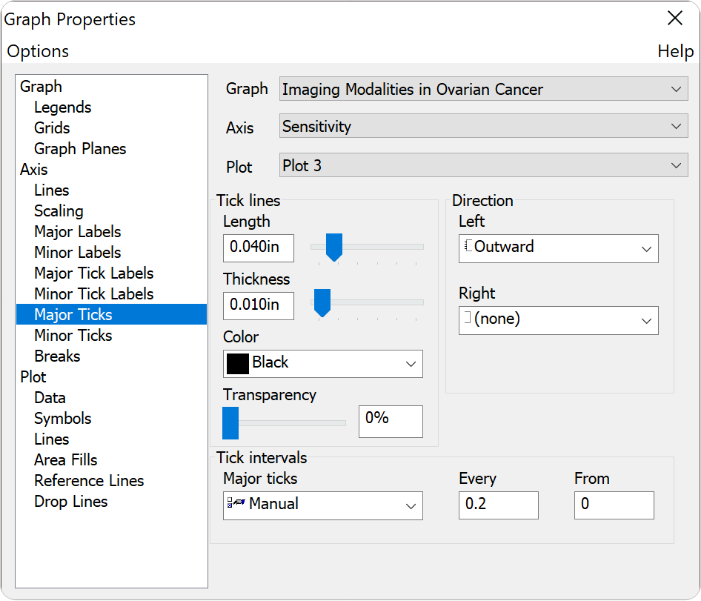
With the new Graph Properties user interface you can select the property category in the tree on the left and then change properties on the right. The change is immediately graphed and if you move your cursor off the panel then it becomes transparent and you can see the effect of your changes without leaving the panel.
The “select left and change right” procedure makes editing your graphs quick and easy. SigmaPlot takes you beyond simple spreadsheets to help you show off your work clearly and precisely. With SigmaPlot, you can produce high-quality graphs without spending hours in front of a computer. SigmaPlot offers seamless Microsoft Office® integration, so you can easily access data from Microsoft Excel® spreadsheets and present your results in Microsoft PowerPoint® presentations.
The user interface also includes Microsoft Office style ribbon controls. And the tabbed window interface efficiently organizes your worksheets and graphs for easy selection. And these tabs may be organized into either vertical or horizontal tab groups. Graph Gallery and Notebook Manger panes may be moved to any position and easily placed using docking panel guides. You can add frequently used objects to the Quick Access Toolbar. For example you might want to add Notebook Save, Close All, Refresh Graph Page and Modify Plot.
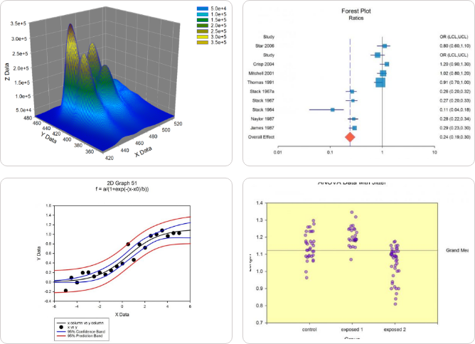
More than 100 2-D and 3-D technical graph type
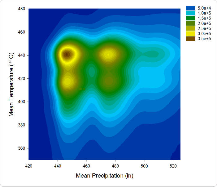
From simple 2-D scatter plots to compelling contour and the new radar and dot density plots, SigmaPlot gives you the exact technical graph type you need for your demanding research.
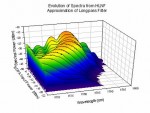
And, to help you see interactions in your 3-D data, SigmaPlot powerfully renders multiple intersecting 3-D meshes with hidden line removal. With so many different chart and graph types to choose from, you can always find the best visual representation of your data.
Use Global Curve Fitting to simultaneously analyze multiple data
Global curve fitting is used when you want to fit an equation to several data sets simultaneously. The selected equation must have exactly one independent variable.
The data sets can be selected from a worksheet or a graph using a variety of data formats. You can also specify the behavior of each equation parameter with respect to the data sets. A parameter can be localized to have a separate value for each data set, or a parameter can be shared to have the same value for all data sets. The Global Curve Fit Wizard is very similar to the Regression and Dynamic Fit Wizards in design and operation. The main difference is the extra panel shown below for specifying the shared parameters.
Obtain Data from Nearly Any Source
SigmaPlot has import file formats for all common text files. This includes a general purpose ASCII file importer which allows importing comma delimited files and user-selected delimiters.
Plus all Excel formats may be imported. SPSS, Minitab, SYSTAT and SAS input data formats are supported by SigmaPlot. Axon binary and text electrophysiology files may be imported. Also the Electrophysiology module, purchased separately, allows importing specific parts of electrophysiology files from Axon Instruments ABF files, Bruxton Corporation’s Acquire format and HEKA electronik’s Pulse format. Import any ODBC compliant database. Excel and Access database files are supported. Run SQL queries on tables and selectively import information.
SigmaPlot Features
Choose from a wide range of graph types to best present your results
From simple 2-D scatter plots to compelling contour and the new radar and dot density plots, SigmaPlot gives you the exact technical graph type you need for your demanding research.
And, to help you see interactions in your 3-D data, SigmaPlot powerfully renders multiple intersecting 3-D meshes with hidden line removal. With so many different chart and graph types to choose from, you can always find the best visual representation of your data.
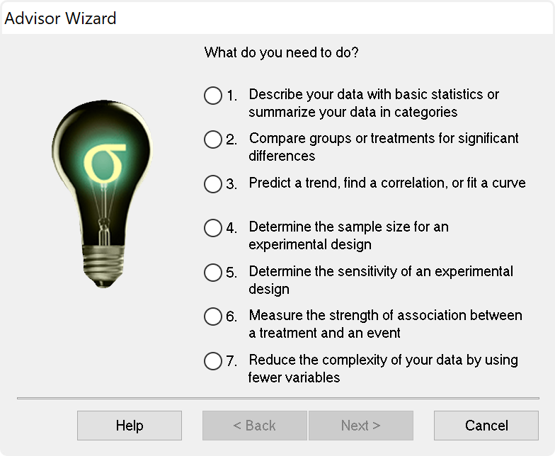
Statistical Analysis is no longer a daunting task
SigmaPlot now offers almost 50 of the most frequently used statistical tests in scientific research by integrating SigmaStat into one application. Suggestion of the most appropriate statistical tests is offered by a software-based Advisor. Raw and indexed data formats are accepted to avoid data reformatting.
Violation of data assumptions is checked in the background and, if true, the correct test to use is recommended. Reports with descriptive interpretations are generated and graphs specific to each test may be created.
SigmaPlot now employs an all new user interface allowing users to easily setup a global curve fit. This gives users the ability to easily share one or more equation parameters across multiple data sets.
Non-linear curve fitting is known to produce incorrect results in some instances.The problem is that you don´t necessarily know that this has happened. Dynamic Curve Fitting is designed to determine if this has happened and if so what the likely best fit is.
Share high-quality graphs and data on the Web
Export your graphs as high-resolution, dynamic Web pages – not simple GIF or JPEG files. Viewers can explore data used to create graphs and zoom, pan or print images at full resolution directly from a Web Browser. Automatically generate active Web objects from your graphs or embed the objects within other Web pages.
- Simply select the Web graph to share its data with colleagues and students
- Share the data behind your graphs with colleagues and students
- Enable colleagues to print your full report from your intranet or Web site directly from their browsers – without compromising the quality of the graphs
- Create an optional password while exporting your graph to limit data access to authorized users
- Produce Web documents without knowing HTML or embed SigmaPlot Web object graphs within HTML files to create interactive electronic reports
Each worksheet can hold a list of user defined transforms that will automatically be re-run whenever the transform input data has changed.
Let’s say you would like to start by selecting a particular kind of graph but you don’t know how to set up the worksheet to achieve it. SigmaPlot lets the user select a graph first and then gives you a pre-formatted worksheet to structure their data. The data entered into the worksheet is immediately displayed on the graph. This feature can demonstrate to you the strong relationship between the data format and the graph type.
Import
- Excel, ASCII Plain Text, Comma Delimited, MS Access
- General ASCII import filter
- SigmaPlot DOS 4.0, 4.1, 5.0 data worksheets, SigmaPlot 1.0, 2.0 Worksheet, and 3.0, 4.0, 5.0, 6.0, 7.0, 8.0, 9.0, 10.0 and 11.0 Windows, SigmaPlot 4.1 and 5.0 Macintosh data worksheets
- Comma delimited and general purpose ASCII import filter
- Symphony, Quattro Pro, dBASE E, DIF, Lotus 1-2-3, Paradox
- SigmaStat DOS and 1.0 worksheets, SYSTAT, SPSS, SAS data set V6. V8, V9, SAS export file, Minitab V8 to V12
- SigmaScan, SigmaScan Pro, SigmaScan Image, Mocha
- TableCurve 2D and 3D
- Axon Binary, Axon Text
- Import ODBC compliant databases
- Run SQL queries on tables and selectively import information
- Import Excel 2007 files directly into SigmaPlot
Export
- Excel, ASCII Plain Text, Comma Delimited, MS Access
- General ASCII import filter
- SigmaPlot DOS 4.0, 4.1, 5.0 data worksheets, SigmaPlot 1.0, 2.0 Worksheet, and 3.0, 4.0, 5.0, 6.0, 7.0, 8.0, 9.0, 10.0 and 11.0 Windows, SigmaPlot 4.1 and 5.0 Macintosh data worksheets
- Comma delimited and general purpose ASCII import filter
- Symphony, Quattro Pro, dBASE E, DIF, Lotus 1-2-3, Paradox
- SigmaStat DOS and 1.0 worksheets, SYSTAT, SPSS, SAS data set V6. V8, V9, SAS export file, Minitab V8 to V12
- SigmaScan, SigmaScan Pro, SigmaScan Image, Mocha
- TableCurve 2D and 3D
- Axon Binary, Axon Text
- Import ODBC compliant databases
- Run SQL queries on tables and selectively import information
- Import Excel 2007 files directly into SigmaPlot
Graphing software that makes data visualization easy
Graph creation starts with SigmaPlot’s award-winning interface. Take advantage of ribbon collections of common properties, tabbed selection of graphs, worksheets and reports, right mouse button support and graph preferences. Select the graph type you want to create from the Graph Toolbar’s easy-to-read icons. The interactive Graph Wizard leads you through every step of graph creation. You get compelling, publication-quality charts and graphs in no time. SigmaPlot offers more options for charting, modeling and graphing your technical data than any other graphics software package.
Compare and contrast trends in your data by creating multiple axes per graph, multiple graphs per page and multiple pages per worksheet. Accurately arrange multiple graphs on a page using built-in templates or your own page layouts with SigmaPlot’s WYSIWYG page layout and zoom features.
Customize every detail of your charts and graphs
SigmaPlot offers the flexibility to customize every detail of your graph. You can add axis breaks, standard or asymmetric error bars and symbols; change colors, fonts, line thickness and more. Double-click on any graph element to launch the Graph Properties dialog box. Modify your graph, chart or diagram further by pasting an equation, symbol, map, picture, illustration or other image into your presentation. And select anti-aliasing to display jaggy-free smooth lines that can be used in your PowerPoint® presentations.
Quickly Plot your Data from Existing Graph Templates in the Graph Style Gallery
Save all of the attributes of your favorite graph style in the Graph Style Gallery. Add greater speed and efficiency to your analysis by quickly recalling an existing graph type you need and applying its style to your current dataset.
- Quickly save any graph with all graph properties as a style and add a bitmap image to the gallery
- No need to be an expert, create customized graphs in no time with the Graph Gallery
- Choose an image from the Graph Style Gallery to quickly plot your data using an existing graph template
- Save time by using a predetermined style to create a graph of the data
- Avoid re-creating complex graphs
But, remember, you don’t necessarily need to use the power of the Graph Gallery since every graph in SigmaPlot is a template. In the Notebook Manager, you can copy and paste a graph from one worksheet to another and all the attributes of that graph are applied to the new data saving much time.
Publish your charts and graphs anywhere
Create stunning slides, display your graphs in reports or further customize your graphs in drawing packages. Save graphs for publication in a technical journal, article or paper with SigmaPlot’s wide range of graphic export options. Presenting and publishing your results has never been easier – or looked this good.
Create customized reports with SigmaPlot’s Report Editor or embed your graphs in any OLE (Object Linking and Embedding) container – word processors, Microsoft PowerPoint or another graphics program. Then, just double click your graph to edit directly inside your document. Quickly send your high-resolution graphs online to share with others.
Data Analysis Doesn’t Get Much Easier
SigmaPlot provides all the fundamental tools you need to analyze your data from basic statistics to advanced mathematical calculations. Click the View Column Statistics button to instantly generate summary statistics including 95% and 99% confidence intervals. Run t-tests, linear regressions, non-linear regressions and ANOVA with ease. You can fit a curve or plot a function and get a report of the results in seconds. Use built-in transforms to massage your data and create a unique chart, diagram or figure. With SigmaPlot – it’s all so simple!
Use SigmaPlot within Microsoft Excel
Access SigmaPlot right from your active Microsoft Excel worksheet. Tedious cut-and-paste data preparation steps are eliminated when you launch SigmaPlot’s Graph Wizard right from the Excel toolbar. Use Excel in-cell formulas, pivot tables, macros and date or time formats without worry. Keep your data and graphs in one convenient file.
Transforms and Quick Transforms
Generate simulated data or modify worksheet columns of data with transforms. Create simple one-line transforms with the Quick Transforms feature that walks you through transform implementation. Or create extremely complex transforms with hundreds of lines of code.
Use the Regression Wizard to fit data easily and accurately
Fitting your data is easy with the SigmaPlot Regression Wizard. The Regression Wizard automatically determines your initial parameters, writes a statistical report, saves your equation to your SigmaPlot Notebook, and adds your results to existing graphs or creates a new one!
The Regression Wizard accurately fits nearly any equation – piecewise continuous, multifunctional, weighted, Boolean functions and more – up to 10 variables and 25 parameters. You can even add your own curve fit equations and add them to the Regression Wizard.
Use the Dynamic Curve Fitter to determine if your fit is valid
The Dynamic Curve Fitter performs 200 or more curve fits using your equation and data starting from optimally different initial starting values. The results are ranked by goodness of fit so that you can check the top ranked results against the result you obtained from the Regression Wizard.
For many simple equations, which are fit to data sets with a sufficiently large number of data points, the Dynamic Curve Fitter finds the same result as the Regression Wizard. But the problem is that the user simply does not know whether the solution found by the Regression Wizard is the best possible or not. So there is always a concern that the correct solution has not been found. Dynamic fitting minimizes this concern. Its use is encouraged prior to publishing results particularly if a complicated equation is used.
Plot Nearly ANY Mathematical Function
Plotting user-defined and parameterized equations is only a mouseclick away with the Plot Equation feature. Just type the function or select one from the built-in library and specify the parameters and the range. It’s that simple! Create your own built-in functions and save them for future use. Plot functions on new or existing graphs or plot multiple functions simultaneously using different parameter values. Save plotted X and Y results to the worksheet.
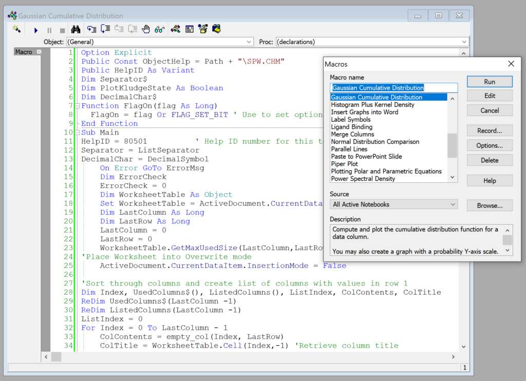
Maximize your Productivity with SigmaPlot’s Automation
Automate Complex Repetitive Tasks
Create macros in no time with SigmaPlot’s easy-to-use macro language. Not a programmer? No problem. With SigmaPlot, you can record macros by point-and-click with the macro recorder. Use macros to acquire your data, execute powerful analytical methods, and create industry-specific or field-specific graphs. Use one of the thirty built-in macros as provided or use these macros as a base to quickly create your own macros.
Share the power of SigmaPlot with less-experienced users by using macros to tailor the SigmaPlot interface for your particular application. Create custom dialog boxes, menu choices and forms to help guide novice users through a session.
Call on SigmaPlot´s functionality from external sources that have Visual Basic embedded including Microsoft Word®, Microsoft Excel®, Microsoft PowerPoint® or custom software applications. Analyze and graph your data using SigmaPlot within those applications.
For example, you can run a Visual Basic script in Microsoft Word® or Excel® that calls on SigmaPlot to generate and embed your graph in the document. SigmaPlot´s OLE2 automation provides unlimited flexibility.
SigmaPlot Has Complete Advisory Statistical Analysis Features
SigmaPlot is now a complete graphing AND an advisory statistics suite. All of the advanced statistical analysis features found in the package known as SigmaStat have now been incorporated into SigmaPlot along with several new statistical features. SigmaPlot guides users through every step of the analysis and performs powerful statistical analysis without the user being a statistical expert.
In addition to the EC50 value already computed, the user can also compute other user-entered EC values such as EC40 and EC60 and compute them instantly. Two five-parameter logistic functions have also been added and the Dynamic Curve Fitting feature included to help solve difficult curve fitting problems.
In earlier versions of SigmaPlot, almost all objects in a 2D graph were selectable with just a mouse click. However, almost all objects in a 3D graph were not. SigmaPlot now adds mouse selectability of all 3D graph objects with the ability to customize all 3D objects.
New Worksheet Features Include
- Import Excel worksheet data into a SigmaPlot worksheet or Open an Excel worksheet as an Excel worksheet in SigmaPlot
- Mini toolbar for worksheet cell editing
- Zoom enabled worksheet
- Worksheet scrolling with mouse wheel
- Line widths may be placed in the worksheet for graph customization
- Formatted text (subscript, etc.) in worksheet cells
Create stunning slides, display your graphs in reports or further customize your graphs in drawing packages. Save graphs for publication in a technical journal, article or paper with SigmaPlot’s wide range of graphic export options. Presenting and publishing your results has never been easier – or looked this good. Create customized reports with SigmaPlot’s Report Editor or embed your graphs in any OLE container – word processors, Microsoft PowerPoint or graphics program. Just double click your graph to edit directly inside your document. Quickly send your high-resolution graphs online to share with others.
SigmaPlot’s Notebook Functionality
- Can hold SigmaPlot worksheets, Excel worksheets, reports, documents, regression wizard equations, graph pages, and macros.
- New dialog-bar-based notebook that has several states: docks, re-sizable, hide-able, summary information mode, etc.
- Browser-like notebook functionality that supports drag-n-drop capabilities
- Direct-editing of notebook summary information
Automate Routine and Complex Tasks
- Visual Basic compatible programming using built-in macro language interface
- Macro recorder to save and play-back operations
- Full automation object support – use Visual Basic to create your own SigmaPlot-based applications
- Run built-in macros or create and add your own scripts
- Add menu commands and create dialog boxes
- Toolbox ribbon: helpful macros appear as separate grouped items
- Export graph to PowerPoint Slide (macro)
- “Insert Graph to Microsoft Word” Toolbox ribbon macro
- Keyboard shortcuts in the Graph page and most Microsoft Excel keyboard shortcuts in the worksheet.
Symbol Types
- Over 100 symbol types
- 30 new symbol types that include half-filled and BMW styles
- Edit font when using text as symbol
- Access new symbols directly from graph properties dialog, toolbar, legend page and the symbol dialog box
- More line types such as dash and gap patterns
- More fill patterns for bar charts and area plots, that can be independently set from the line color
SigmaPlot Report Editor
- Cut and paste or use OLE to combine all the important aspects of your analysis into one document.
- Copy / Paste tabular data between report and Excel worksheet
- Choose from a wide range of styles, sizes and colors from any system font
- New tables with pre-defined styles or user customized
- Export to most word processors
- Add decimal tabs, tab leader, true date/time fields
- Vertical and horizontal rulers for report formatting
- Auto-numbering
- Change report background color
- Improved formatting ruler
- Zoom enabled in reports
- Drag and drop Word 2007 and 2010 documents into reports
Page Layout and Annotation Options
- OLE 2 container and server
- Automatic or manual legends
- True WYSIWYG
- Multi line text editor
- Multiple curves and plots on one graph
- Multiple axes on one graph
- Arrange graphs with built-in templates
- Multiple levels of zooming and custom zooming
- Scale graph to any size
- Resize graphic elements proportionally with resizing graph
- Alignment and position tools
- Draw lines, ellipses, boxes, arrows
- Layering options
- Over 16 million custom colors
- Inset graphs inside one another
- Selection of graph objects
- Right-click property editing
- New zoom, drag and pan controls
- Mouse wheel scrolling enabled
- Right-click property editing for 3D Graphs
- Color schemes
- Paste graphic objects from other